Description
Stock prices — and even their cumulative returns — often show long-term upward or downward trends that can mask underlying behavior. This can cause some misinterpretation of the true seasonal trend of the underlying instrument. In this post, we’ll use Python to calculate the yearly cumulative returns of a stock, understand what this metric really means, and then detrend the return series to reveal its true fluctuations and relative performance over time. This is a follow-up article from the seasonal trend analysis done for AMZN in the previous article here.
Now, we’ll walk through how to compute cumulative returns for the time period, why detrending is essential, and how to use Python to uncover the true shape of a stock’s performance.
What Are Cumulative Returns?
Cumulative return measures how much an investment grows over a period relative to its starting value.
For example:
- If AMZN starts the year at $100 and ends at $150
→ The yearly cumulative return is +50%.
Looking at cumulative returns over the full historical period helps visualize:
- The path of returns (not just the final result)
- How gains or losses accumulate
- How volatile or smooth the returns accumulate over the years
The cumulative returns have a limitation:
Long-term growth produces an upward drift, making the search for a seasonal trend across years difficult. This is where detrending helps.
Calculating Yearly Cumulative Returns
We’ll use yfinance to download AMZN daily prices and calculate daily percentage changes.
Python Example
import yfinance as yf
import pandas as pd
import matplotlib.pyplot as plt

amzn= yf.Ticker("AMZN")
data = amzn.history(period='25y',interval='1d', auto_adjust=False)

data['Return'] = data['Adj Close'].pct_change()
data['DayOfYear'] = data.index.dayofyear
# Compute average daily returns by calendar day
avg_daily = data.groupby('DayOfYear')['Return'].mean()
cum_avg = avg_daily.cumsum()
This gives us a nice per-day cumulative return path from the last 25 years.
Why Detrend the Cumulative Return Line
Stocks like AMZN have:
- long-term uptrends
- increasingly large price moves
- compounding effects
These factors cause later years to appear more volatile or stronger simply because the stock is bigger.
Detrending removes the long-term drift and lets us see the cumulative returns and seasonal pattern more consistent.
How to Detrend Cumulative Returns
There are multiple detrending approaches, such as:
- subtracting a linear trend
- dividing by the year’s ending return
- z-scaling (standardization)
- subtracting a polynomial trend
For simplicity and clarity, we’ll detrend the cumulative returns by removing their long-term moving average.
This isolates the shape of the return path, independent of its magnitude.
Python Example:
sma_250 = cum_avg.rolling(window=250, min_periods=1).mean()

# Detrend the cumulative average returns by subtracting the SMA
# We use .dropna() to handle initial NaN values from the rolling mean calculation if needed
detrended_cum_avg = cum_avg - sma_250
In this example, we calculate the 250-day Simple Moving Average (SMA) of the cumulative returns. For detrending, the SMA is typically applied to the original time series to estimate the trend component, which is then subtracted from the original cumulative line.
Visualizing the Result
Here are example plots you can generate:
# Plotting
plt.figure(figsize=(10,6))
plt.plot(cum_avg, label='Cumulative Avg Daily Return (AMZN)', color='blue')
plt.plot(detrended_cum_avg, label='Detrended Cumulative Avg Daily Return (SMA 250)', color='orange', linestyle='--')
plt.title('Amazon Seasonality Pattern (2000–Present)')
plt.xlabel('Day of Year')
plt.ylabel('Cumulative Average Return')
plt.legend()
plt.grid(True)
plt.show()
This shows how much returns drift upward over time.
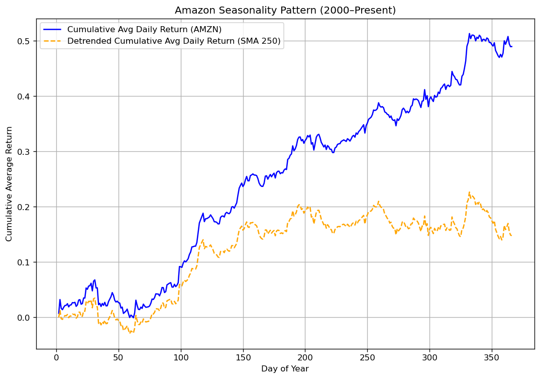
Now, all years have a similar baseline.
The benefit: underlying performance shapes become visible:
- strong early-year trends
- mid-year volatility
- late-year reversals
- changes in momentum patterns over decades
Detrending transforms what was previously noise-covered data into an analyzable pattern.
Final Thoughts
Cumulative returns are one of the most intuitive ways to visualize stock performance throughout a year, but their upward drift can mask the story beneath the surface. By detrending the series, we reveal the true structure of returns and can compare performance patterns across decades on equal footing.
This method is especially useful when:
- researching seasonal tendencies
- building systematic strategies
- comparing regime changes
- identifying consistent return shapes
- removing bias caused by long-term growth
In future posts, we’ll apply detrending to multiple assets at once and examine how stable these intrayear shapes really are — and whether they offer a tradable edge.
This is the mindset behind The Quantitative Edge — simple ideas, implemented cleanly, that scale into powerful tools for data-driven trading.
Statemi bene!