Description
In my previous article on Seasonal Trading using Amazon (AMZN), I explored how recurring market behaviors can reveal a quiet but measurable edge. Now, let’s take the same approach to a broader level — analyzing the S&P 500 ETF (SPY) to uncover how the market itself tends to move across the calendar year.
This time, I am not reintroducing the concept or code — if you missed the first article, you can find the full Python workflow and description here.
Now the focus is on the results, the interpretation, and the insights from the monthly seasonality profile of SPY.
From Daily Returns to Monthly Patterns
Using the same methodology — daily percentage returns from Yahoo Finance — we aggregate returns by month and calculate two key statistics for each one:
- Average Daily % Change – How strong or weak that month typically is.
- % of Positive Years – How consistently that month has produced positive returns over the years.
The Python implementation builds directly on the previous article and can be extended as follows:
import yfinance as yf
import matplotlib.pyplot as plt
import pandas as pd

t = yf.Ticker("SPY")
spy = t.history(start="2000-01-01",interval='1d', auto_adjust=False)

spy['Month'] = spy.index.month
spy['Year'] = spy.index.year

spy['Daily Return'] = spy['Adj Close'].pct_change()

monthly_returns = spy.groupby(['Year', 'Month'])['Daily Return'].mean().reset_index()

avg_return = monthly_returns.groupby('Month')['Daily Return'].mean()

# Compute % of positive months
positive_ratio = monthly_returns.groupby('Month')['Daily Return'].apply(lambda x: (x > 0).mean() * 100)

monthly_stats = pd.DataFrame({
    'Avg Daily % Change': avg_return * 100,
    '% Positive Years': positive_ratio
})

month_names = ['January', 'February', 'March', 'April', 'May', 'June',
               'July', 'August', 'September', 'October', 'November', 'December']
monthly_stats.index = month_names

# Plot side-by-side bar chart
fig, ax1 = plt.subplots(figsize=(10, 6))

ax1.bar(monthly_stats.index, monthly_stats['Avg Daily % Change'], color='steelblue', alpha=0.7, label='Avg Daily % Change')

ax2 = ax1.twinx()
ax2.plot(monthly_stats.index, monthly_stats['% Positive Years'], color='darkorange', marker='o', label='% Positive Years')

ax1.set_title('SPY Monthly Seasonality — Average Daily % Change and % Positive Years')
ax1.set_ylabel('Avg Daily % Change (%)')
ax2.set_ylabel('% of Positive Years')
ax1.set_xticklabels(monthly_stats.index, rotation=45)
ax1.grid(axis='y', linestyle='--', alpha=0.6)

lines, labels = ax1.get_legend_handles_labels()
lines2, labels2 = ax2.get_legend_handles_labels()
ax1.legend(lines + lines2, labels + labels2, loc='upper left')

plt.tight_layout()
plt.show()
We then visualize these results in a combined chart:
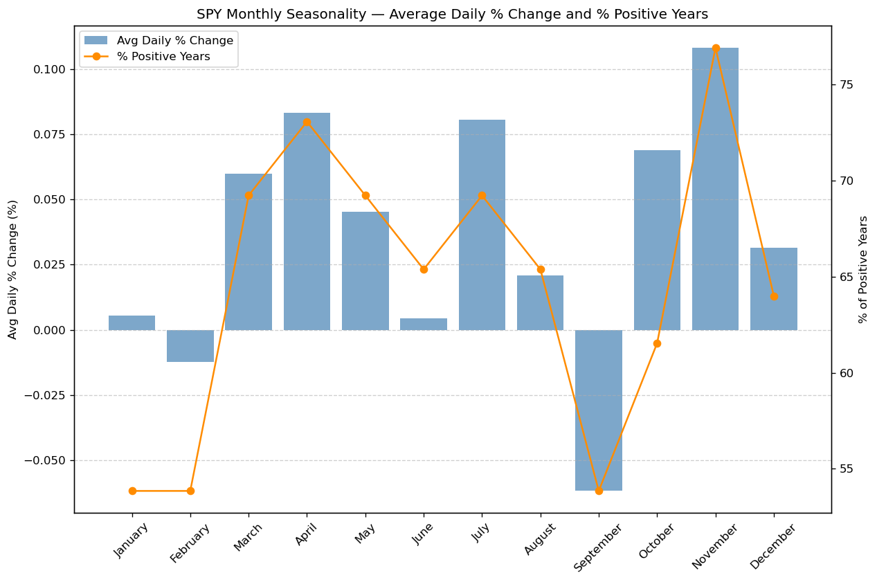
The blue bars represent the average daily return per month. The orange line indicates the frequency of positive months since 2000.
Seasonality Results for SPY
From the chart, several key observations stand out:
- Strongest months: November, December, and April.
These months show both higher average returns and strong consistency (over 75% of years positive).
Historically, this period captures the post-earnings optimism and year-end inflows. - Weaker months: August and September.
Returns here are often flat or negative, and the probability of a positive outcome drops sharply — reflecting lower liquidity and risk aversion during summer. - Transition phases: March and October often act as turning points — volatility increases, but so does opportunity.
October, despite its reputation for crashes, is often the setup month for the strong November–December rally.
Why This Matters
This simple monthly breakdown already gives structure to market randomness. It highlights when the market tends to reward risk, and when patience or reduced exposure pays off.
A systematic trader can use this information to:
- Align portfolio exposure with favorable months.
- Adjust position sizing or leverage depending on seasonal strength.
- Validate whether a trading system performs consistently across these historical seasonal boundaries.
From Patterns to Trades
Once a seasonal pattern is statistically confirmed, the next step is trading it efficiently. Take, for example, the recurring bullish window from late October to mid-December.
There are several practical ways to position for it:
- Buying the shares directly:
The most straightforward approach — entering a long SPY position at the start of the window and closing near mid-December. This method benefits from the average upward drift and can be enhanced by position sizing or stop-loss rules. - Using options to trade:
A trader can implement either a bull call spread (buying a call and selling a higher-strike call) or a bull put spread (selling a put and buying a lower-strike put). Both express a moderately bullish view but define risk and capital use more efficiently. The expiration should align with the end of the seasonal window, while the strike distance should roughly reflect the historical average gain of the pattern — for instance, a 5 % spread if the seasonality historically averages 5 % upside.
These techniques convert statistical tendencies into structured, risk-managed trades — the core of systematic seasonal investing.
Final Thoughts
Seasonal analysis offers a powerful way to look beyond daily noise and uncover the market’s recurring behavior.
By understanding when performance clusters — like SPY’s consistent strength between late October and mid-December — traders can align their strategies with long-term statistical tendencies instead of short-term emotions.
However, as with any quantitative edge, validation and robustness are key. A strong seasonal pattern must prove itself across multiple years, and ideally across related markets or indices.
Only then does it become a reliable component of a systematic trading playbook.
From here, the natural next step is to explore option-based implementations — where spreads, expirations, and strike selections are chosen to reflect the strength and timing of these patterns.
That’s exactly what we’ll dive into in the upcoming article.
This is the mindset behind The Quantitative Edge — simple ideas, implemented cleanly, that scale into powerful tools for data-driven trading.
Statemi bene!