Description
Every market headline mentions it. “Fear gauge spikes.” “Volatility collapses.” Yet most traders who watch the VIX every day could not tell you what it is made of.
That is a problem if you sell options. The VIX is not a sentiment indicator. It is a price. Specifically, it is the price the market is charging today for 30 days of S&P 500 uncertainty, extracted directly from SPX option quotes.
If you sell premium, you are on the other side of that price. Understanding how it is built, how it behaves, and how it compares to the volatility that actually shows up afterwards is one of the cleanest edges available to a retail options trader.
In this article I will cover three things. What the VIX actually is, from first principles. Where to download the data, with Python code that works. And how I use it in my own trading, for the Wheel and for the seasonal bull put spreads.
Introduction: The Week the VIX Crossed 30
On March 27, 2026, the VIX closed at 31.05. Three weeks earlier it had been hovering around 20. If you read the April newsletter, you know how that month felt: the S&P 500 down more than 4%, small caps worse, and my Wheel portfolio sitting on a painful drawdown.
Here is the interesting part. That same week, the premium I could collect on a put spread was the richest I had seen all year. My Greedy Brain loved it. My Risk Management Brain wanted to close the laptop. My Systematic Brain asked the only useful question: what is the VIX actually telling me, and what has it historically meant?
Thirteen days later, on April 9, the VIX closed at 19.49. The fear had been repriced in less than two weeks. Traders who understood what the VIX is, and how fast it mean-reverts, sold that fear. Traders who treated it as a headline sold their stocks instead.
This article is the framework I use to tell the two situations apart.
What the VIX Actually Measures
The VIX is the market’s expectation of S&P 500 volatility over the next 30 calendar days, expressed as an annualized percentage. A VIX of 20 means option prices imply roughly 20% annualized volatility for the index.
The important word is implied. Nobody votes on the VIX. Cboe computes it from live SPX option prices, using a published methodology:
- Take the two SPX expirations that bracket 30 days: one with more than 23 days left, one with less than 37. Both standard monthly and Friday weekly expirations are eligible.
- For each expiration, take every out-of-the-money put and call around the forward price, using the mid of bid and ask. Stop when two consecutive strikes have a zero bid.
- Turn that strip of options into a variance number, one per expiration.
- Interpolate the two variances to exactly 30 days, annualize, take the square root, multiply by 100.
For each expiration, step 3 is this formula:
$$\sigma^2 = \frac{2}{T} \sum_i \frac{\Delta K_i}{K_i^2} e^{RT} Q(K_i) - \frac{1}{T} \left( \frac{F}{K_0} - 1 \right)^2$$
Don’t let it scare you. As a physicist I read it like this: it is a weighted sum over the whole option chain, where each option price Q(K) is weighted by 1/K². Cheap far-OTM puts get a large weight. That is the key insight most traders miss.
The VIX is not the at-the-money implied volatility. It includes the wings, and in equity markets the wings are the downside puts. So when portfolio managers rush to buy crash protection, the VIX jumps even if ATM volatility barely moves. That is why it earned the nickname “fear gauge”: it literally prices the demand for insurance.
From VIX to Expected Move
The most practical thing you can do with the VIX is convert it into an expected move. Volatility scales with the square root of time, so:
$$\text{30-day 1}\sigma\text{ move} \approx \frac{\text{VIX}}{\sqrt{12}} \qquad \text{daily 1}\sigma\text{ move} \approx \frac{\text{VIX}}{\sqrt{252}} \approx \frac{\text{VIX}}{16}$$
The second one is the famous rule of 16. A VIX of 16 means the market is pricing a typical daily move of about 1%. A VIX of 32 means about 2% a day.
(Note: In the options market, 365 calendar days is standard for pricing models, though some traders substitute 252 trading days depending on the specific platform).
import numpy as np

def expected_move(vix, spx, days=30):
    """1-sigma expected move of SPX implied by the VIX."""
    sigma = vix / 100 * np.sqrt(days / 365)
    return sigma * 100, spx * sigma

for vix in [12, 16, 20, 25, 31.05]:
    pct, pts = expected_move(vix, spx=6500)
    print(f"📊 VIX {vix:>5}: ±{pct:4.1f}% in 30 days (±{pts:,.0f} SPX points)")
Output:
📊 VIX    12: ± 3.4% in 30 days (±224 SPX points)
📊 VIX    16: ± 4.6% in 30 days (±298 SPX points)
📊 VIX    20: ± 5.7% in 30 days (±373 SPX points)
📊 VIX    25: ± 7.2% in 30 days (±466 SPX points)
📊 VIX 31.05: ± 8.9% in 30 days (±579 SPX points)
The SPX level of 6,500 is just a round number for the example. Change it to today’s price.
Two caveats before we move on. First, this is a risk-neutral number: it includes the insurance premium, so it systematically overstates what usually happens. We will measure that gap below. Second, you cannot buy the VIX itself. VIX futures and VIX options settle on the future value of the index, which is a different animal.
Where to Get VIX Data (For Free)
Good news: the VIX is one of the easiest datasets in finance to get. The bad news: every source has a quirk. Here is what I use and why.
| Source | What you get | History | Best for |
|---|---|---|---|
| Cboe VIX historical data | Official daily OHLC as a CSV | Close from 1990, OHLC from 1992 | The reference series, straight from the source |
| FRED VIXCLS | Daily close only | From 1990 | Clean, stable URL, perfect for scripts |
yfinance (^VIX, ^VIX9D, ^VIX3M, ^VIX6M) |
Daily OHLC for the VIX family | Varies by ticker | Term structure in one line of Python |
| Cboe Futures Exchange | VIX futures settles, one CSV per contract | From 2004 | Futures curve and roll yield research |
| Interactive Brokers API | Live and intraday VIX, futures, options | Depends on subscription | Execution-time decisions |
A note on history. Cboe changed the VIX formula on September 22, 2003. The values before that date were back-calculated with the new methodology, so the series is consistent, but remember the market structure of 1995 was very different from today. For options work I usually start my analysis in 2004, when VIX futures began trading and the volatility market matured. Macroption keeps a good overview of these details.
VIX options history is the exception: it is not free. If you need it, Cboe DataShop or a commercial vendor is the way.
A Robust Python Loader
Cboe’s website changes often, and links break. So I always load the official CSV with a fallback to FRED:
import pandas as pd

CBOE_URL = "https://cdn.cboe.com/api/global/us_indices/daily_prices/VIX_History.csv"
FRED_URL = "https://fred.stlouisfed.org/graph/fredgraph.csv?id=VIXCLS"

def load_vix():
    """Daily VIX close. Cboe first, FRED as fallback."""
    try:
        df = pd.read_csv(CBOE_URL, index_col=0, parse_dates=True)
        vix = df["CLOSE"]
        print("✅ Loaded VIX from Cboe")
    except Exception:
        df = pd.read_csv(FRED_URL, index_col=0, parse_dates=True)
        vix = pd.to_numeric(df["VIXCLS"], errors="coerce")
        print("⚠️ Cboe unavailable, loaded VIX from FRED")
    vix = vix.dropna().rename("VIX")
    print(f"📅 {vix.index[0]:%Y-%m-%d} → {vix.index[-1]:%Y-%m-%d}, {len(vix):,} days")
    return vix

vix = load_vix()
FRED marks holidays with a dot instead of a number, which is why the to_numeric with errors="coerce" is there. Skip it and your whole column becomes text.
For the term structure, yfinance is the shortest path:
import yfinance as yf

tickers = ["^VIX9D", "^VIX", "^VIX3M", "^VIX6M"]
term = yf.download(tickers, start="2011-01-01", progress=False)["Close"].dropna()
term.columns = [c.replace("^", "") for c in term.columns]
print(term.tail(3).round(2))
VIX9D, VIX, VIX3M and VIX6M are the same calculation applied to 9 days, 30 days, 3 months and 6 months of SPX options. Put them side by side and you have the volatility curve for free.
Three Patterns Hiding in the VIX Data
Now the fun part. With 20+ years of daily data, three properties of the VIX jump out. Each one has a direct consequence for how you sell options.
Pattern 1: The VIX Is Skewed, Not Normal
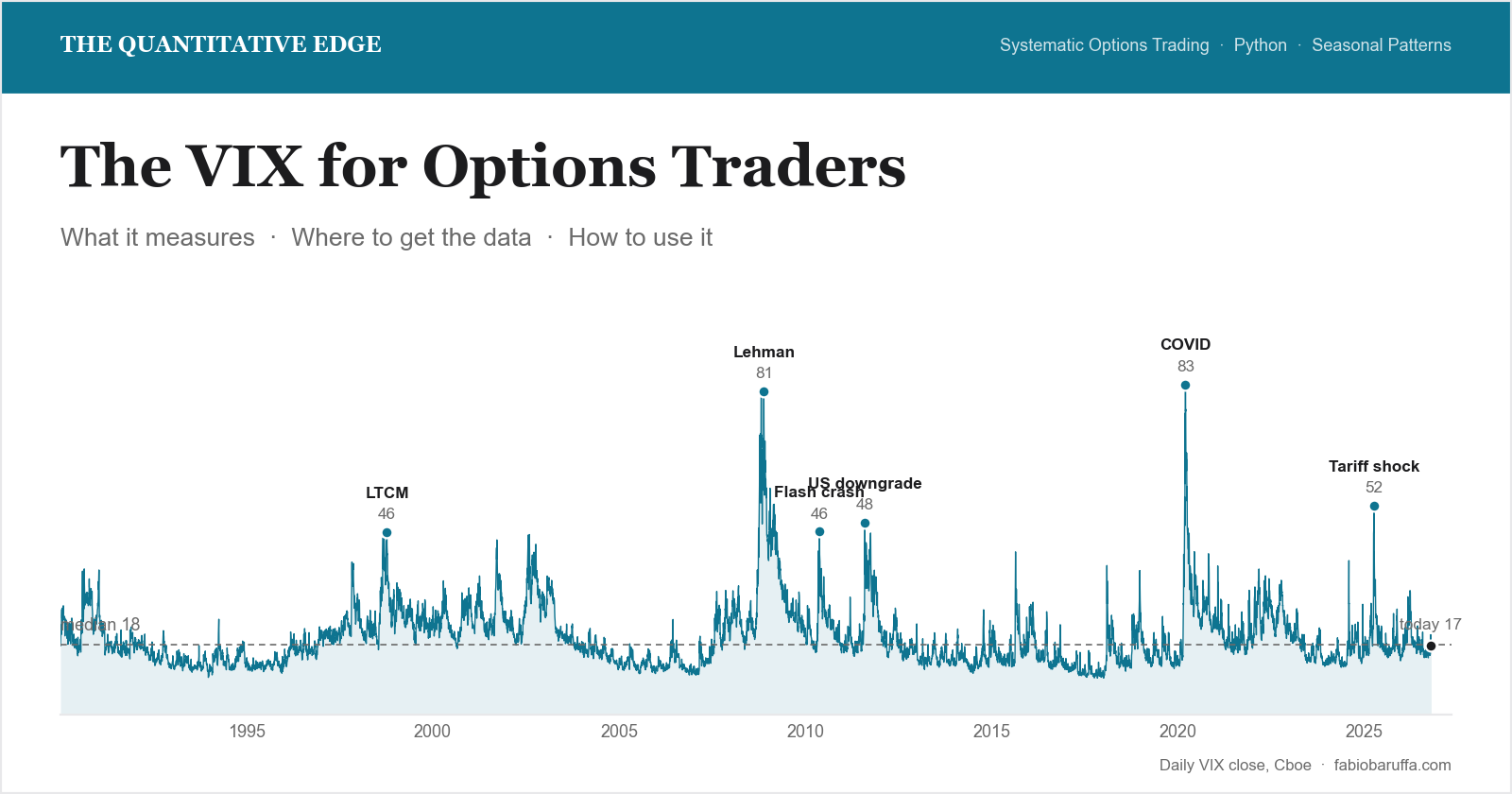
The VIX has a floor and no ceiling. Its all-time intraday high is 89.53, set in October 2008, and its record close is 82.69 on March 16, 2020. On the low side, it rarely spends time below 10. So the distribution is heavily right-skewed: long calm stretches, interrupted by short violent spikes.
This means the average VIX is a misleading number. Use percentiles.
v = vix.loc["2004":]

print(f"📊 Mean:   {v.mean():.1f}")
print(f"📊 Median: {v.median():.1f}")
for q in [0.10, 0.25, 0.75, 0.90, 0.95]:
    print(f"📏 {int(q*100):>2}th percentile: {v.quantile(q):.1f}")
print(f"🔥 Days above 30: {(v > 30).mean():.1%}")
Output:
✅ Loaded VIX from Cboe
📅 1990-01-02 → 2026-10-20, 9,298 days
📊 Mean:   18.9
📊 Median: 16.6
📏 10th percentile: 12.0
📏 25th percentile: 13.6
📏 75th percentile: 21.6
📏 90th percentile: 27.9
📏 95th percentile: 33.5
🔥 Days above 30: 7.8%
The mean sits clearly above the median. That gap is the skew: a handful of crisis months pull the average up. When someone tells you “the VIX is above its average”, check the percentile instead. A VIX of 20 can be perfectly normal.
For reference, the yearly average close on FRED was 25.6 in 2022, 16.9 in 2023, 15.6 in 2024 and 18.9 in 2025. Same index, very different regimes.
Pattern 2: The VIX Mean-Reverts, Fast
Stock prices can trend for years. The VIX cannot. Fear is expensive to maintain, and spikes tend to decay as the market digests the shock. March 2026 was a textbook example: 31.05 on March 27, 19.49 on April 9.
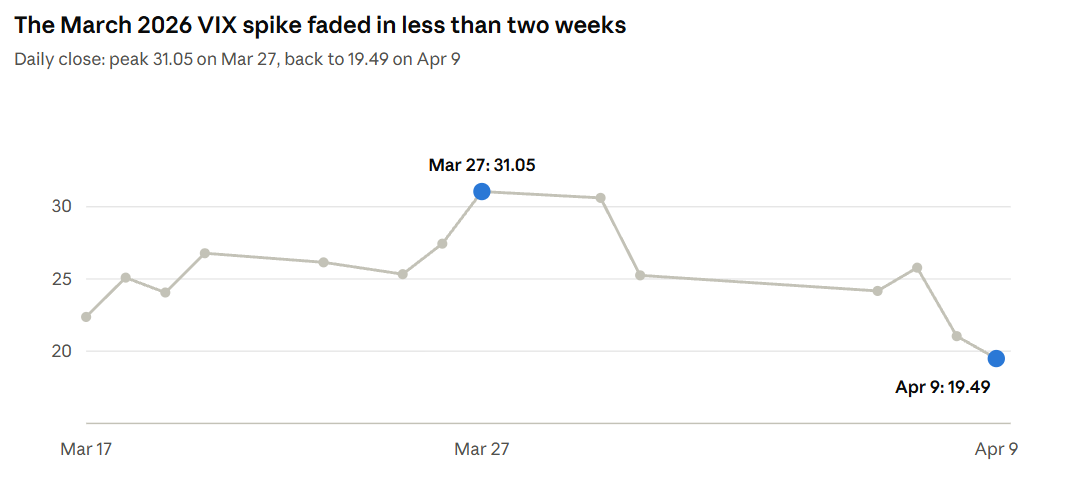
A 31 became a 19 in eight trading sessions. No news made the world safe in that time. The insurance simply got repriced.
A physicist’s way to measure this is the half-life of a shock. Fit a simple AR(1) model on the log of the VIX, and convert the coefficient into days:
import numpy as np

log_v = np.log(v)
dx = log_v.diff().dropna()
x_prev = log_v.shift(1).dropna().loc[dx.index]

b = np.polyfit(x_prev, dx, 1)[0]          # slope of the mean-reversion
half_life = -np.log(2) / np.log(1 + b)

print(f"🔁 Mean-reversion coefficient: {b:.4f}")
print(f"⏳ Half-life of a VIX shock: {half_life:.0f} trading days")
Output:
🔁 Mean-reversion coefficient: -0.0224
⏳ Half-life of a VIX shock: 31 trading days
The exact number depends on the sample, but the conclusion does not: shocks fade in weeks, not years. This is why short-duration option structures make sense after a spike. You are selling insurance at a price that the data says will not last.
One warning. Mean reversion tells you where the VIX tends to go, not when. In late 2008 it stayed above 40 for weeks on end. That is why sizing matters more than timing.
Pattern 3: Implied Beats Realized, Most of the Time
This is the most important pattern for a premium seller. Compare the VIX on each day with the volatility the S&P 500 actually delivered over the following 21 trading days.
import yfinance as yf

spx = yf.download("^GSPC", start="2004-01-01", progress=False)["Close"].squeeze()
ret = np.log(spx).diff()

# realized vol over the NEXT 21 trading days, annualized, in VIX points
realized = ret.rolling(21).std().shift(-21) * np.sqrt(252) * 100

df = pd.concat([v, realized.rename("RV")], axis=1).dropna()
df["VRP"] = df["VIX"] - df["RV"]

print(f"💰 Average VIX - realized: {df['VRP'].mean():+.1f} vol points")
print(f"✅ Days VIX > realized: {(df['VRP'] > 0).mean():.0%}")
print(f"💥 Worst miss: {df['VRP'].min():+.1f} on {df['VRP'].idxmin():%Y-%m-%d}")
Output:
💰 Average VIX - realized: +3.5 vol points
✅ Days VIX > realized: 84%
💥 Worst miss: -69.9 on 2020-02-19
That spread has a name: the variance risk premium. Option buyers pay for insurance, and like every insurance business, the seller collects a premium on average. This is the structural edge behind the Wheel, the cash-secured put, and every credit spread on this blog.
But look at the worst miss. On a few days, realized volatility blew far past what the VIX had priced. The premium seller wins small and often, and loses big and rarely. That asymmetry is the whole game. The VIX does not remove it. It helps you decide when the premium is worth the risk.
How I Use the VIX as an Options Trader
I do not use the VIX to predict the market. I use it to answer two practical questions before every trade. Is premium cheap or expensive right now? And is the market calm, or stressed?
Level: Is Premium Worth Selling?
The level, ranked against its own history, tells me how much insurance is paying. I never look at the raw number alone. I look at its percentile over the last few years:
def vix_percentile(vix, window=252 * 3):
    """Where today's VIX sits within the last 3 years, from 0 to 100."""
    return vix.rolling(window).rank(pct=True) * 100

pct = vix_percentile(vix)
print(f"🎯 VIX today: {vix.iloc[-1]:.2f}, percentile: {pct.iloc[-1]:.0f}")
Output:
🎯 VIX today: 17.31, percentile: 63
A low percentile means thin premium: I sell less, or further out of the money. A high percentile means rich premium, which is exactly when the Greedy Brain gets loud.
Term Structure: Calm or Stressed?
The level alone is not enough. A VIX of 25 can be a buying opportunity or the beginning of a crash. The term structure tells the two apart.
In normal markets, longer-dated volatility is higher than short-dated: VIX3M sits above VIX. This is called contango, and it is the market saying “things are fine now, but who knows in three months”. In a panic, the curve flips. Short-term fear becomes more expensive than long-term fear, and VIX rises above VIX3M. That is backwardation.
ratio = term["VIX"] / term["VIX3M"]

state = np.where(ratio > 1.0, "🔴 Backwardation: stress",
         np.where(ratio > 0.9, "🟡 Flat: caution", "🟢 Contango: calm"))

print(f"📐 VIX / VIX3M = {ratio.iloc[-1]:.3f} → {state[-1]}")
print(f"📊 Share of days in backwardation since 2011: {(ratio > 1).mean():.0%}")
This ratio is one of the three lenses in my market regime framework, and it is the one that reacted first during the 2026 correction. The 0.9 threshold is a reasonable starting point, not a magic number. Test it on your own data.
Putting It Together
Combine the two lenses and you get four situations, each with a different response:
| VIX percentile | Term structure | What it means | What I do |
|---|---|---|---|
| Low | Contango | Calm and cheap | Sell small, far OTM, or wait |
| High | Contango | Fear is fading, premium is rich | The sweet spot: sell defined-risk premium |
| High | Backwardation | Active panic | Defense only: no new short exposure |
| Low | Backwardation | Rare, often the start of a shock | Reduce size, tighten stops |
The exact sizing rules I use for each regime are in How I Use Market Regimes to Size My Option Trades. Here I want to focus on the reasoning.
Go back to the end of March 2026. The VIX was above 31 and my screen was red. My three brains had a short conversation.
Greedy Brain: “Premium hasn’t been this rich all year. Sell everything!”
Risk Management Brain: “Spikes like this come with an inverted curve. Realized volatility can still blow past implied. One bad week and the drawdown doubles.”
Systematic Brain: “Check the term structure, not the headline. Backwardation means no new short exposure. Contango with an elevated VIX is the signal. And whatever you sell, the risk must be defined.”
That is the logic behind the seasonal bull put spreads I traded on MCD and HAS this spring: rich premium, a statistical edge from SeasonHunter, small size, and defined risk on every position. No naked exposure while the VIX was screaming.
For Wheel Traders
The Wheel is a short-volatility strategy in disguise. Every cash-secured put you sell is a small insurance contract on a single stock. So the VIX matters even if you never trade an index option.
When the VIX is low, I am pickier on strikes and stock selection, because the premium does not pay for mistakes. When it spikes, single-stock implied volatility usually spikes even more, and the puts on quality names become attractive. That is exactly when the free cash flow filter earns its keep: high premium on a stock you are happy to own is the Wheel at its best.
Final Thoughts
The VIX is not a fear index. It is a price tag. It tells you what the market is charging for 30 days of S&P 500 uncertainty, built from the whole SPX option chain, with a heavy weight on the downside puts.
Once you see it that way, three things follow. It is skewed, so read it in percentiles, not averages. It mean-reverts, so spikes are opportunities for those who survive them. And it usually overprices what actually happens, which is the structural reason premium selling works at all.
The flip side is just as important. The VIX underprices the rare disaster, and that is where premium sellers get destroyed. The term structure is your early warning. Respect backwardation, keep risk defined, and size so that the worst miss in your backtest does not end your trading career.
The data is free. The code is above. Download it, run it on your own sample, and look at the numbers yourself. That is the only way the pattern becomes yours.
If you have questions or want to share what you found, send me a message. I read every one.
This is the mindset behind The Quantitative Edge — simple ideas, implemented cleanly, that scale into powerful tools for data-driven trading.
Stammi bene!